Hierarchical Reasoning Model
階層的推論モデル

Contact: research@sapient.inc.
Code available at: github.com/sapientinc/HRM

Abstract　要旨

Reasoning, the process of devising and executing complex goal-oriented action sequences, remains a critical challenge in AI. Current large language models (LLMs) primarily employ Chain-of-Thought (CoT) techniques, which suffer from brittle task decomposition, extensive data requirements, and high latency. Inspired by the hierarchical and multi-timescale pro- cessing in the human brain, we propose the Hierarchical Reasoning Model (HRM), a novel recurrent architecture that attains signifcant computational depth while maintaining both train- ing stability and effciency. HRM executes sequential reasoning tasks in a single forward pass without explicit supervision of the intermediate process, through two interdependent recurrent modules: a high-level module responsible for slow, abstract planning, and a low-level mod- ule handling rapid, detailed computations. With only 27 million parameters, HRM achieves exceptional performance on complex reasoning tasks using only 1000 training samples. The model operates without pre-training or CoT data, yet achieves nearly perfect performance on challenging tasks including complex Sudoku puzzles and optimal path fnding in large mazes. Furthermore, HRM outperforms much larger models with signifcantly longer context windows on the Abstraction and Reasoning Corpus (ARC), a key benchmark for measuring artifcial general intelligence capabilities. These results underscore HRM's potential as a transformative advancement toward universal computation and general-purpose reasoning systems.
推論は、複雑な目標指向のアクションシーケンスを考案して実行するプロセスであり、AI において依然として重要な課題です。現在の大規模言語モデル (LLM) は主に思考連鎖(Chain-of-Thought(CoT)) 手法を採用していますが、タスク分解が不安定で、データ要件が膨大で、レイテンシが高いという問題があります。人間の脳の階層的でマルチタイムスケールの処理にヒントを得て、我々は階層的推論モデル (HRM) を提案します。これは、トレーニングの安定性と効率性の両方を維持しながら、大きな計算深度を実現する新しい再帰型アーキテクチャです。HRM は、2 つの相互に依存する再帰型モジュール (低速で抽象的な計画を担当する高レベルモジュールと、高速で詳細な計算を処理する低レベルモジュール) を介して、中間プロセスの明示的な監視なしに、単一のフォワードパスで順次推論タスクを実行します。わずか 2,700 万のパラメーターで、HRM はわずか 1,000 のトレーニング サンプルを使用して複雑な推論タスクで並外れたパフォーマンスを実現します。このモデルは事前学習やCoTデータなしで動作し、複雑な数独パズルや大規模迷路における最適経路探索といった難解なタスクにおいてほぼ完璧なパフォーマンスを達成しています。さらに、HRMは、汎用人工知能の能力を測定するための重要なベンチマークである抽象化推論コーパス（ARC）において、はるかに長いコンテキストウィンドウを持つ、はるかに大規模なモデルよりも優れた性能を発揮します。これらの結果は、HRMが普遍的な計算および汎用推論システムに向けた革新的な進歩となる可能性を強く示唆しています。

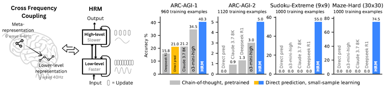
Figure 1: Left: HRM is inspired by hierarchical processing and temporal separation in the brain. It has two recurrent networks operating at different timescales to collaboratively solve tasks. Right: With only about 1000 training examples, the HRM (~27M parameters) surpasses state-of-the-art CoT models on inductive benchmarks (ARC-AGI) and challenging symbolic tree-search puzzles (Sudoku-Extreme, Maze-Hard) where CoT models failed completely. The HRM was randomly initialized, and it solved the tasks directly from inputs without chain of thoughts.
図1：左：HRMは、脳内の階層的処理と時間的分離に着想を得ています。異なる時間スケールで動作する2つのリカレントネットワークが協調的にタスクを解決します。右：わずか1000件の学習例で、HRM（約2700万パラメータ）は、最先端のCoTモデルを、帰納的ベンチマーク（ARC-AGI）と、CoTモデルが完全に失敗した難解な記号木探索パズル（Sudoku-Extreme、Maze-Hard）で凌駕します。HRMはランダムに初期化され、思考の連鎖なしに入力から直接タスクを解決しました。

1. Introduction　はじめに

Deep learning, as its name suggests, emerged from the idea of stacking more layers to achieve increased representation power and improved performance^1,2. However, despite the remarkable success of large language models, their core architecture is paradoxically shallow³. This imposes a fundamental constraint on their most sought-after capability: reasoning. The fxed depth of stan- dard Transformers places them in computational complexity classes such as \(AC^0\) or \(TC^0\)⁴, prevent- ing them from solving problems that require polynomial time^5,6. LLMs are not Turing-complete and thus they cannot, at least in a purely end-to-end manner, execute complex algorithmic rea- soning that is necessary for deliberate planning or symbolic manipulation tasks^7,8. For example, our results on the Sudoku task show that increasing Transformer model depth can improve per- formance,¹ but performance remains far from optimal even with very deep models (see Figure 2 ), which supports the conjectured limitations of the LLM scaling paradigm⁹.
ディープラーニングは、その名前が示すように、より多くのレイヤーを積み重ねることで表現力を高め、パフォーマンスを改善するというアイデアから生まれました^1,2。しかし、大規模言語モデルの目覚ましい成功にもかかわらず、そのコアアーキテクチャは逆説的に浅いものです³。これが、最も求められている機能である推論に根本的な制約を課しています。標準的なTransformerの固定された深さは、\(AC^0\)や\(TC^0\)⁴などの計算複雑性クラスに分類され、多項式時間を必要とする問題を解くことができません^5,6。LLMはチューリング完全ではないため、少なくとも純粋にエンドツーエンドでは、意図的な計画や記号操作タスクに必要な複雑なアルゴリズム推論を実行できません^7,8。たとえば、数独タスクの結果では、Transformer モデルの深さを増やすとパフォーマンスが向上することがわかりました ¹ が、非常に深いモデルでもパフォーマンスは最適にはほど遠いままです (図 2 を参照)。これは、LLM スケーリング パラダイムの想定される限界を裏付けています ⁹。

¹ Simply increasing the model width does not improve performance here.
モデルの幅を単に増やすだけではパフォーマンスは向上しません。

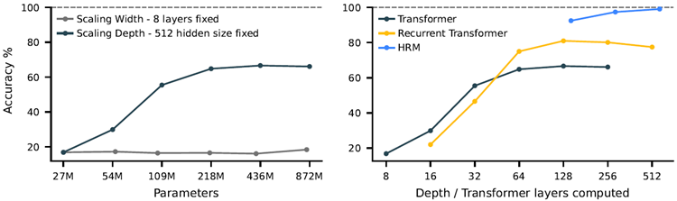
Figure 2: The necessity of depth for complex reasoning. Left: On Sudoku-Extreme Full, which require extensive tree-search and backtracking, increasing a Transformer's width yields no perfor- mance gain, while increasing depth is critical. Right: Standard architectures saturates, failing to beneft from increased depth. HRM overcomes this fundamental limitation, effectively using its computational depth to achieve near-perfect accuracy.
図2：複雑な推論における深さの必要性。左：膨大なツリー探索とバックトラッキングを必要とするSudoku-Extreme Fullでは、Transformerの幅を広げてもパフォーマンスは向上せず、深さを増やすことが重要である。右：標準的なアーキテクチャは飽和状態になり、深さの増加によるメリットが得られない。HRMはこの根本的な限界を克服し、計算深さを効果的に活用してほぼ完璧な精度を実現している。

The LLMs literature has relied largely on Chain-of-Thought (CoT) prompting for reasoning¹⁰. CoT externalizes reasoning into token-level language by breaking down complex tasks into sim- pler intermediate steps, sequentially generating text using a shallow model¹¹. However, CoT for reasoning is a crutch, not a satisfactory solution. It relies on brittle, human-defned decompositions where a single misstep or a misorder of the steps can derail the reasoning process entirely^12,13. This dependency on explicit linguistic steps tethers reasoning to patterns at the token level. As a result, CoT reasoning often requires signifcant amount of training data and generates a large number of tokens for complex reasoning tasks, resulting in slow response times. A more effcient approach is needed to minimize these data requirements¹⁴.
LLMの文献は、推論において主に思考連鎖（CoT）の促進に依存してきました¹⁰。CoTは、複雑なタスクをより単純な中間ステップに分解し、浅いモデルを用いて逐次テキストを生成することで、推論をトークンレベルの言語に外在化します¹¹。しかし、推論のためのCoTは松葉杖であり、満足のいく解決策ではありません。CoTは、人間が定義した脆弱な分解に依存しており、1つのステップの誤りやステップの順序の誤りが推論プロセス全体を狂わせる可能性があります^12,13。明示的な言語ステップへの依存は、推論をトークンレベルのパターンに縛り付けます。その結果、CoT推論は多くの場合、大量のトレーニングデータを必要とし、複雑な推論タスクに対して多数のトークンを生成するため、応答時間が遅くなります。これらのデータ要件を最小限に抑えるには、より効率的なアプローチが必要です¹⁴。

Towards this goal, we explore “latent reasoning”, where the model conducts computations within its internal hidden state space^15,16. This aligns with the understanding that language is a tool for human communication, not the substrate of thought itself¹⁷; the brain sustains lengthy, coherent chains of reasoning with remarkable effciency in a latent space, without constant translation back to language. However, the power of latent reasoning is still fundamentally constrained by a model's effective computational depth. Naively stacking layers is notoriously diffcult due to vanishing gra- dients, which plague training stability and effectiveness^1,18. Recurrent architectures, a natural al- ternative for sequential tasks, often suffer from early convergence, rendering subsequent computa- tional steps inert, and rely on the biologically implausible, computationally expensive and memory intensive Backpropagation Through Time (BPTT) for training¹⁹.
この目標に向けて、我々は「潜在的推論」を探求しています。これは、モデルが内部の隠れ状態空間内で計算を行うものです^15,16。これは、言語は人間のコミュニケーションのためのツールであり、思考そのものの基盤ではないという理解と一致しています¹⁷。脳は潜在空間において、言語への絶え間ない翻訳なしに、長く一貫した推論の連鎖を驚くべき効率で維持します。しかし、潜在的推論の能力は、依然としてモデルの有効な計算深度によって根本的に制約されています。単純に層を積み重ねることは、勾配消失のために非常に困難であり、トレーニングの安定性と有効性に悪影響を及ぼします^1,18。逐次タスクの自然な代替手段である再帰型アーキテクチャは、多くの場合、早期収束に悩まされ、後続の計算ステップが不活性化され、生物学的に不可能で、計算コストが高く、メモリを大量に消費する Backpropagation Through Time (BPTT) に依存してトレーニングを行っています¹⁹。

The human brain provides a compelling blueprint for achieving the effective computational depth that contemporary artifcial models lack. It organizes computation hierarchically across corti- cal regions operating at different timescales, enabling deep, multi-stage reasoning^20,21,22. Recur- rent feedback loops iteratively refne internal representations, allowing slow, higher-level areas to guide, and fast, lower-level circuits to execute—subordinate processing while preserving global coherence^23,24,25. Notably, the brain achieves such depth without incurring the prohibitive credit- assignment costs that typically hamper recurrent networks from backpropagation through time^19,26.
人間の脳は、現代の人工モデルに欠けている効果的な計算深度を実現するための魅力的な青写真を提供します。脳は、異なる時間スケールで動作する皮質領域にわたって階層的に計算を組織化し、深く多段階の推論を可能にします^20,21,22。再帰フィードバックループは内部表現を反復的に洗練させ、低速で高レベルの領域が誘導し、高速で低レベルの回路が実行することを可能にします。これにより、全体的な一貫性を維持しながら、従属的な処理が可能になります^23,24,25。注目すべきは、脳がこのような深度を、通常、時間経過による逆伝播からの再帰ネットワークの計算を阻害する法外なクレジット割り当てコストを負担することなく実現している点です^19,26。

Inspired by this hierarchical and multi-timescale biological architecture, we propose the Hierar- chical Reasoning Model (HRM). HRM is designed to signifcantly increase the effective compu- tational depth. It features two coupled recurrent modules: a high-level (H) module for abstract, deliberate reasoning, and a low-level (L) module for fast, detailed computations. This structure avoids the rapid convergence of standard recurrent models through a process we term “hierarchi- cal convergence.” The slow-updating H-module advances only after the fast-updating L-module has completed multiple computational steps and reached a local equilibrium, at which point the L-module is reset to begin a new computational phase.
この階層的かつマルチタイムスケールの生物学的構造に着想を得て、我々は階層的推論モデル（HRM）を提案する。HRMは、実効的な計算深度を大幅に向上させるように設計されている。HRMは、抽象的で慎重な推論を行う高レベル（H）モジュールと、高速で詳細な計算を行う低レベル（L）モジュールという、2つの結合した回帰モジュールを特徴とする。この構造は、「階層的収束」と呼ぶプロセスを通じて、標準的な回帰モデルに見られる急速な収束を回避する。更新速度の遅いHモジュールは、更新速度の速いLモジュールが複数の計算ステップを完了して局所平衡に達した後にのみ前進し、その時点でLモジュールはリセットされ、新たな計算フェーズを開始する。

Furthermore, we propose a one-step gradient approximation for training HRM, which offers im- proved effciency and eliminates the requirement for BPTT. This design maintains a constant mem- ory footprint (O(1) compared to BPTT's O(T) for T timesteps) throughout the backpropagation process, making it scalable and more biologically plausible.
さらに、HRMの学習に1ステップ勾配近似法を提案する。これにより効率が向上し、BPTTが不要になる。この設計により、バックプロパゲーション処理全体を通してメモリ使用量が一定（TタイムステップのBPTTのO(T)と比較してO(1)）に維持されるため、スケーラブルで生物学的妥当性も向上する。

Leveraging its enhanced effective depth, HRM excels at tasks that demand extensive search and backtracking. Using only 1,000 input-output examples, without pre-training or CoT supervision, HRM learns to solve problems that are intractable for even the most advanced LLMs. For example, it achieves near-perfect accuracy in complex Sudoku puzzles (Sudoku-Extreme Full) and optimal pathfnding in 30x30 mazes, where state-of-the-art CoT methods completely fail (0% ac- curacy). In the Abstraction and Reasoning Corpus (ARC) AGI Challenge^27,28,29 - a benchmark of inductive reasoning - HRM, trained from scratch with only the offcial dataset (~1000 exam- ples), with only 27M parameters and a 30x30 grid context (900 tokens), achieves a performance of 40.3%, which substantially surpasses leading CoT-based models like o3-mini-high (34.5%) and Claude 3.7 8K context (21.2%), despite their considerably larger parameter sizes and con- text lengths, as shown in Figure 1 . This represents a promising direction toward the development of next-generation AI reasoning systems with universal computational capabilities.
HRMは、強化された有効深度を活用することで、広範な探索とバックトラッキングを必要とするタスクにおいて優れた性能を発揮します。わずか1,000個の入出力例を使用し、事前学習やCoTによる監督なしに、HRMは最先端のLLMでさえ解くことが困難な問題を学習します。例えば、複雑な数独パズル（Sudoku-Extreme Full）においてほぼ完璧な精度を達成し、最先端のCoT手法では完全に失敗する（精度0%）30x30迷路における最適経路探索を実現します。帰納的推論のベンチマークである抽象化および推論コーパス（ARC）AGIチャレンジ^27,28,29において、公式データセット（約1000例）のみ、わずか2700万のパラメータ、30x30グリッドコンテキスト（900トークン）でゼロからトレーニングされたHRMは、40.3％のパフォーマンスを達成しました。これは、図1に示すように、パラメータサイズとコンテキスト長がかなり大きいにもかかわらず、o3-mini-high（34.5％）やClaude 3.7 8Kコンテキスト（21.2％）などの主要なCoTベースのモデルを大幅に上回っています。これは、普遍的な計算能力を備えた次世代AI推論システムの開発に向けた有望な方向性を示しています。

2 Hierarchical Reasoning Model 階層的推論モデル

We present the HRM, inspired by three fundamental principles of neural computation observed in the brain:
私たちは、脳内で観察される神経計算の 3 つの基本原理に着想を得た HRM を紹介します。

The HRM model consists of four learnable components: an input network \(f_I(·;θ_I)\), a low-level re- current module \(f_L(·;θ_L)\), a high-level recurrent module \(f_H(·;θ_H)\), and an output network \(f_O(·;θ_O)\). The model's dynamics unfold over \(N\) high-level cycles of \(T\) low-level timesteps each². We index the total timesteps of one forward pass by \(i = 1, . . . , N×T\). The modules \(f_L\) and \(f_H\) each keep a hidden state—\(z_L^i\) for \(f_L\) and \(z_H^i\) for \(f_H\)—which are initialized with the vectors \(z_L^0\) and \(z_H^0\), respectively.
HRMモデルは、学習可能な4つのコンポーネントで構成されています。入力ネットワーク\(f_I(·;θ_I)\)、低レベルリカレントモジュール\(f_L(·;θ_L)\)、高レベルリカレントモジュール\(f_H(·;θ_H)\)、および出力ネットワーク\(f_O(·;θ_O)\)です。モデルのダイナミクスは、\(T\)個の低レベルタイムステップをそれぞれ2回繰り返す\(N\)個の高レベルサイクルにわたって展開されます。1回のフォワードパスの合計タイムステップは、\(i = 1, . . . , N×T\)でインデックス付けされます。モジュール \(f_L\) と \(f_H\) はそれぞれ隠れ状態 (\(f_L\) の場合は \(z_L^i\)、\(f_H\) の場合は \(z_H^i\)) を保持し、これらはそれぞれベクトル \(z_L^0\) と \(z_H^0\) で初期化されます。

² While inspired by temporal separation in the brain, our model's “high-level” and “low-level” modules are conceptual abstractions and do not map directly to specifc neural oscillation frequencies.
私たちのモデルの「高レベル」および「低レベル」モジュールは、脳内の時間的分離にヒントを得ていますが、概念的な抽象化であり、特定の神経振動周波数に直接マッピングされるわけではありません。

The HRM maps an input vector \(x\) to an output prediction vector \(\hat{y}\) as follows. First, the input \(x\) is projected into a working representation \(\tilde{x}\) by the input network:
HRMは、入力ベクトル\(x\)を出力予測ベクトル\(\hat{y}\)に以下のようにマッピングします。まず、入力\(x\)は入力ネットワークによって作業表現\(\tilde{x}\)に投影されます。 \[ \tilde{x} = f_I(x;θ_I) \] At each timestep \(i\), the \(L\)-module updates its state conditioned on its own previous state, the \(H\)- module's current state (which remains fxed throughout the cycle), and the input representation. The H-module only updates once per cycle (i.e., every \(T\) timesteps) using the \(L\)-module's fnal state at the end of that cycle:
各タイムステップ \(i\) において、\(L\) モジュールは、自身の前回の状態、\(H\) モジュールの現在の状態（サイクルを通して固定）、および入力表現に基づいて状態を更新します。H モジュールは、サイクルごとに（つまり、\(T\) タイムステップごとに）1 回のみ、そのサイクルの終了時の \(L\) モジュールの最終状態を使用して更新します。 \[ \begin{align} z_L^i &= f_L(z_L^{i−1}, z_H^{i−1},\tilde{x};θ_L) \\ \\ z_H^i &= \begin{cases} f_H(z_H^{i-1},z_L^{i-1},\theta_H) &if\;i\equiv0\;(mod\;T) \\ \\ z_H^{i-1} & otherwise \end{cases} \end{align} \] Finally, after \(N\) full cycles, a prediction \(\hat{y}\) is extracted from the hidden state of the \(H\)-module:
最後に、\(N\)回の完全なサイクルの後、\(H\)モジュールの隠れ状態から予測\(\hat{y}\)が抽出されます。 \[ \hat{y} = f_O(z_H^{NT};θ_O) \] This entire \(NT\)-timestep process represents a single forward pass of the HRM. A halting mecha- nism (detailed later in this section) determines whether the model should terminate, in which case \(\hat{y}\) will be used as the fnal prediction, or continue with an additional forward pass.
この \(NT\)-タイムステッププロセス全体は、HRM の単一のフォワードパスを表します。停止メカニズム（このセクションで後述）によって、モデルを終了するかどうかが決定されます。終了した場合は \(\hat{y}\) が最終予測として使用されます。終了しない場合は、追加のフォワードパスが実行されます。

Hierarchical convergence　Although convergence is crucial for recurrent networks, standard RNNs are fundamentally limited by their tendency to converge too early. As the hidden state settles toward a fxed point, update magnitudes shrink, effectively stalling subsequent computation and capping the network's effective depth. To preserve computational power, we actually want convergence to proceed very slowly–but engineering that gradual approach is diffcult, since pushing convergence too far edges the system toward instability.
階層的収束　収束は再帰型ネットワークにとって極めて重要ですが、標準的なRNNは、収束が早すぎるという傾向によって根本的に限界があります。隠れ状態が固定点に向かって落ち着くと、更新量は減少し、後続の計算が事実上停止し、ネットワークの有効な深さが制限されます。計算能力を維持するためには、実際には収束を非常にゆっくりと進める必要がありますが、収束を過度に進めるとシステムが不安定になるため、そのような段階的なアプローチを設計することは困難です。

HRM is explicitly designed to counteract this premature convergence through a process we term hierarchical convergence. During each cycle, the \(L\)-module (an RNN) exhibits stable convergence to a local equilibrium. This equilibrium, however, depends on the high-level state \(z_H\) supplied during that cycle. After completing the \(T\) steps, the \(H\)-module incorporates the sub-computation's outcome (the fnal state \(z_L\)) and performs its own update. This \(z_H\) update establishes a fresh context for the \(L\)-module, essentially “restarting” its computational path and initiating a new convergence phase toward a different local equilibrium.
HRMは、階層的収束と呼ばれるプロセスを通じて、この早期収束を抑制するように明示的に設計されています。各サイクルにおいて、\(L\)モジュール（RNN）は局所平衡点への安定した収束を示します。ただし、この収束点は、そのサイクル中に提供される高レベル状態\(z_H\)に依存します。\(T\)ステップを完了すると、\(H\)モジュールはサブ計算の結果（最終状態\(z_L\)）を取り込み、独自の更新を実行します。この\(z_H\)の更新により、\(L\)モジュールに新たなコンテキストが確立され、実質的に計算パスが「再起動」され、異なる局所平衡点に向けた新たな収束フェーズが開始されます。

This process allows the HRM to perform a sequence of distinct, stable, nested computations, where the \(H\)-module directs the overall problem-solving strategy and the \(L\)-module executes the intensive search or refnement required for each step. Although a standard RNN may approach convergence within T iterations, the hierarchical convergence benefts from an enhanced effective depth of \(NT\) steps. As empirically shown in Figure 3 , this mechanism allows HRM both to maintain high computational activity (forward residual) over many steps (in contrast to a standard RNN, whose activity rapidly decays) and to enjoy stable convergence. This translates into better performance at any computation depth, as illustrated in Figure 2 .
このプロセスにより、HRM は、一連の明確で安定したネストされた計算を実行できます。\(H\) モジュールは全体的な問題解決戦略を指示し、\(L\) モジュールは各ステップで必要な集中的な検索または改良を実行します。標準的な RNN は T 回の反復で収束に近づく可能性がありますが、階層的な収束は、\(NT\) ステップの有効な深度の向上による恩恵を受けます。図 3 で実証的に示されているように、このメカニズムにより、HRM は (アクティビティが急速に減少する標準的な RNN とは対照的に) 多くのステップにわたって高い計算アクティビティ (順方向残差) を維持し、安定した収束を実現できます。これは、図 2 に示すように、どの計算深度でもパフォーマンスが向上することを意味します。

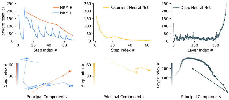
Figure 3: Comparison of forward residuals and PCA trajectories. HRM shows hierarchical conver- gence: the H-module steadily converges, while the L-module repeatedly converges within cycles before being reset by H, resulting in residual spikes. The recurrent neural network exhibits rapid convergence with residuals quickly approaching zero. In contrast, the deep neural network experi- ences vanishing gradients, with signifcant residuals primarily in the initial (input) and fnal layers.
図3：順方向残差とPCA軌跡の比較。HRMは階層的な収束を示している。Hモジュールは着実に収束するのに対し、LモジュールはHによってリセットされる前に周期的に収束を繰り返し、残差にスパイクが生じる。リカレントニューラルネットワークは急速な収束を示し、残差は急速にゼロに近づく。対照的に、ディープニューラルネットワークでは勾配が消失し、主に初期層（入力層）と最終層で大きな残差が生じる。

Approximate gradient　Recurrent models typically use BPTT to compute gradients. However, BPTT requires storing the hidden states from the forward pass and then combining them with gradients during the backward pass, which demands \(O(T)\) memory for T timesteps. This heavy memory burden forces smaller batch sizes and leads to poor GPU utilization, especially for large- scale networks. Additionally, because retaining the full history trace through time is biologically implausible, it is unlikely that the brain implements BPTT¹⁹.
近似勾配　リカレントモデルは通常、勾配を計算するためにBPTTを使用します。しかし、BPTTでは、フォワードパスで隠れ状態を保存し、バックワードパスでそれらを勾配と組み合わせる必要があるため、Tタイムステップで\(O(T)\)のメモリを必要とします。この大きなメモリ負荷により、バッチサイズが小さくなり、特に大規模ネットワークではGPU利用率が低下します。さらに、時間経過を通して完全な履歴トレースを保持することは生物学的に不可能であるため、脳がBPTTを実装している可能性は低いと考えられます¹⁹。

Fortunately, if a recurrent neural network converges to a fxed point, we can avoid unrolling its state sequence by applying backpropagation in a single step at that equilibrium point. Moreover, such a mechanism could plausibly be implemented in the brain using only local learning rules^34,35. Based on this fnding, we propose a one-step approximation of the HRM gradient–using the gradient of the last state of each module and treating other states as constant. The gradient path is, therefore,
幸いなことに、リカレントニューラルネットワークが固定点に収束する場合、その平衡点でバックプロパゲーションを1ステップで適用することで、状態系列の展開を回避できます。さらに、このようなメカニズムは、局所学習規則^34,35のみを用いて脳内に実装できる可能性があります。この発見に基づき、各モジュールの最終状態の勾配を用い、他の状態を一定として扱うことで、HRM勾配の1ステップ近似を提案します。したがって、勾配パスは次のようになります。 \[ \text{Output head → fnal state of the H-module → fnal state of the L-module → input embedding} \] The above method needs \(O(1)\) memory, does not require unrolling through time, and can be easily implemented with an autograd framework such as PyTorch, as shown in Figure 4 . Given that each module only needs to back-propagate errors through its most recent local synaptic activity, this approach aligns well with the perspective that cortical credit assignment relies on short-range, temporally local mechanisms rather than on a global replay of activity patterns.
上記の方法は \(O(1)\) メモリを必要とし、時間軸での展開を必要とせず、図4に示すようにPyTorchなどのautogradフレームワークで簡単に実装できます。各モジュールは最新の局所的なシナプス活動を通じてエラーを逆伝播するだけでよいため、このアプローチは、皮質へのクレジット割り当てが活動パターンのグローバルな再生ではなく、短距離かつ時間的に局所的なメカニズムに依存するという見方とよく一致しています。

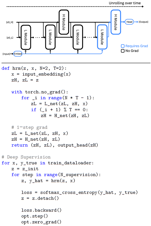
Figure 4: Top: Diagram of HRM with lows us to calculate the exact gradient of fxed point z⋆H approximate gradient. Bottom: Pseu- with respect to the parameters θ without explicit back- docode of HRM with deep supervision propagation:
図4: 上: 固定点z⋆Hの正確な勾配を計算するための近似勾配を用いたHRMの図。下: 明示的な逆伝搬法を用いずに、パラメータθに関する擬似勾配。深層教師伝播を用いたHRMのコード:

The one-step gradient approximation is theoretically grounded in the mathematics of Deep Equilibrium Mod els (DEQ)³⁶ which employs the Implicit Function Theo- rem (IFT) to bypass BPTT, as detailed next. Consider an idealized HRM behavior where, during high-level cycle k, the L-module repeatedly updates until its state \(z_L\) converges to a local fxed point \(z_L^⋆\). This fxed point, given the current high-level state \(z_H^{k−1}\), can be expressed as
1ステップ勾配近似は、理論的には深層平衡モデル（DEQ）³⁶の数学的根拠に基づいており、次に示すように、BPTTを回避するために暗黙関数定理（IFT）を採用しています。高レベルサイクルkにおいて、Lモジュールの状態\(z_L\)が局所的な固定点\(z_L^⋆\)に収束するまで、Lモジュールが繰り返し更新されるという理想的なHRM挙動を考えてみましょう。この固定点は、現在の高レベル状態\(z_H^{k−1}\)が与えられた場合、次のように表すことができます。 \[ z_L^⋆ = f_L(z_L^⋆, z_H^{k−1},\tilde{x};θ_L) \] The \(H\)-module then performs a single update using this converged \(L\)-state:
\(H\)-モジュールは、この収束した \(L\)-状態を使用して単一の更新を実行します。 \[ z_H^k = f_H(z_H^{k−1}, z_L^⋆;θ_H) \] With a proper mapping \(\mathcal{F}\), the updates to the high-level state can be written in a more compact form as \(z_H^k = \mathcal{F}(z_H^{k−1};\tilde{x},θ)\), where \(θ = (θ_I, θ_L)\), and the fxed-point can be written as \(z_H^⋆= \mathcal{F}(zH^⋆;\tilde{x},θ)\). Let \(J_{\mathcal{F}} =\frac{∂\mathcal{F}}{∂z_H}\) be the Jacobian of \(\mathcal{F}\), and assume that the matrix \(I − J_{\mathcal{F}}\) is invertible at \(z_H^⋆\) and that the mapping \(\mathcal{F}\) is continuously differentiable. The Implicit Function Theorem then allows respect to the parameters \(θ\) without explicit backpropagation:
適切なマッピング \(\mathcal{F}\) を用いると、高レベル状態の更新はよりコンパクトな形式で \(z_H^k = \mathcal{F}(z_H^{k−1};\tilde{x},θ)\) と記述できます。ここで \(θ = (θ_I, θ_L)\) であり、固定点は \(z_H^⋆= \mathcal{F}(zH^⋆;\tilde{x},θ)\) と記述できます。 \(J_{\mathcal{F}} =\frac{∂\mathcal{F}}{∂z_H}\) を \(\mathcal{F}\) のヤコビ行列とし、行列 \(I − J_{\mathcal{F}}\) が \(z_H^⋆\) において逆行列を持ち、写像 \(\mathcal{F}\) が連続的に微分可能であると仮定する。すると、暗黙関数定理により、明示的な逆伝播なしにパラメータ \(θ\) に関して以下の式が成立する。 \[ \frac{∂z_H^⋆}{∂θ}=\big(I-J_{\mathcal{F}}\big|_{z_H^*}\big)^{-1}\frac{∂F}{∂θ}\Bigg|_{z_H^*} \tag{1} \] Calculating the above gradient requires evaluating and inverting matrix \((I − J_{\mathcal{F}})\) that can be com- putationally expensive. Given the Neumann series expansion,
上記の勾配を計算するには、行列\((I − J_{\mathcal{F}})\)の評価と逆行列の計算が必要であり、これは計算コストが高くなる可能性がある。ノイマン級数展開を考えると、 \[ (I − J_{\mathcal{F}})^{−1} = I + J_{\mathcal{F}} + J_{\mathcal{F}}^2 + J_{\mathcal{F}}^3 + . . . , \] the so-called 1-step gradient³⁷ approximates the series by considering only its frst term, i.e. \((I − J_{\mathcal{F}})^{−1}\approx I\), and leads to the following approximation of Equation (1):
いわゆる1段階勾配³⁷は、級数をその第1項のみ、つまり\((I − J_{\mathcal{F}})^{−1}\approx I\)を考慮して近似し、式(1)の次の近似値を導きます。 \[ \frac{∂z_H^∗}{∂θ_H}\approx\frac{∂f_H}{∂θ_H},　 \frac{∂z_H^∗}{∂θ_L}\approx\frac{∂f_H}{∂z_L^∗}\cdot\frac{∂z_L^∗}{∂θ_L},　 \frac{∂z_H^∗}{∂θ_I}\approx\frac{∂f_H}{∂z_L^∗}\cdot \frac{∂z_L^∗}{∂θ_I} \tag{2} \] The gradients of the low-level fxed point, \(\frac{∂z_L^∗}{∂θ_L}\) and \(\frac{∂z_K^∗}{∂θ_I}\), can also be approximated using another application of the 1-step gradient:
低レベルの固定点の勾配 \(\frac{∂z_L^∗}{∂θ_L}\) と \(\frac{∂z_K^∗}{∂θ_I}\) も、1 ステップ勾配の別の適用を使用して近似できます。 \[ \frac{∂z_L^∗}{∂θ_L}\approx\frac{∂f_L}{∂θ_L},　\frac{∂z_L^∗}{∂θ_I}\approx\frac{∂f_L}{∂θ_I} \tag{3} \] By substituting Equation (3) back into Equation (2), we arrive at the fnal simplifed gradients.
式(3)を式(2)に代入すると、最終的な簡略化された勾配が得られます。

Before defning our loss function, we must frst introduce two key elements of our proposed method: deep supervision and adaptive computational time.
損失関数を定義する前に、まず、提案方法の 2 つの重要な要素である、深い監視と適応的な計算時間を導入する必要があります。

Deep supervision　Inspired by the principle that periodic neural oscillations regulate when learning occurs in the brain³⁸, we incorporate a deep supervision mechanism into HRM, as detailed next.
ディープスーパービジョン　脳内で学習が起こると周期的な神経振動が制御されるという原理³⁸ に着想を得て、次に詳述するように、ディープスーパービジョンメカニズムを HRM に組み込みました。

Given a data sample \((x, y)\), we run multiple forward passes of the HRM model, each of which we refer to as a segment. Let \(M\) denote the total number of segments executed before termination. For each segment \(m ∈ \{1,..., M\}\), let \(z^m = (z_H^{mNT}, z_L^{mNT})\) represent the hidden state at the conclusion of segment m, encompassing both high-level and low-level state components.
データサンプル \((x, y)\) が与えられた場合、HRM モデルの複数のフォワードパスを実行します。各パスをセグメントと呼びます。\(M\) は、終了までに実行されたセグメントの総数を表します。各セグメント \(m ∈ \{1,..., M\}\) について、\(z^m = (z_H^{mNT}, z_L^{mNT})\) は、セグメント m の終了時の隠れ状態を表し、高レベルと低レベルの両方の状態要素を含みます。

At each segment m, we apply a deep supervision step as follows:
各セグメントmでは、次のように深い監視ステップを適用します。

The crucial aspect of this procedure is that the hidden state \(z^m\) is “detached” from the computa- tion graph before being used as the input state for the next segment. Consequently, gradients from segment \(m + 1\) do not propagate back through segment \(m\), effectively creating a 1-step approxi- mation of the gradient of the recursive deep supervision process^39,40. This approach provides more frequent feedback to the H-module and serves as a regularization mechanism, demonstrating supe- rior empirical performance and enhanced stability in deep equilibrium models when compared to more complex, Jacobian-based regularization techniques^39,41. Figure 4 shows pseudocode of deep supervision training.
この手順の重要な点は、隠れ状態 \(z^m\) が次のセグメントの入力状態として使用される前に、計算グラフから「切り離される」ことです。その結果、セグメント \(m + 1\) からの勾配はセグメント \(m\) を介して伝播せず、再帰的な深層教師プロセスの勾配の1ステップ近似が効果的に作成されます^39,40。このアプローチは、Hモジュールへのフィードバックをより頻繁に提供し、正則化メカニズムとして機能し、より複雑なヤコビアンベースの正則化手法と比較して、深層平衡モデルにおいて優れた経験的パフォーマンスと強化された安定性を示します^39,41。図4は、深層教師トレーニングの疑似コードを示しています。

Adaptive computational time (ACT)　The brain dynamically alternates between automatic think- ing (“System 1”) and deliberate reasoning (“System 2”)⁴². Neuroscientifc evidence shows that these cognitive modes share overlapping neural circuits, particularly within regions such as the prefrontal cortex and the default mode network^43,44. This indicates that the brain dynamically mod- ulates the “runtime” of these circuits according to task complexity and potential rewards^45,46.
適応的計算時間（ACT）　脳は自動思考（「システム1」）と意図的な推論（「システム2」）を動的に切り替えます⁴²。神経科学的な証拠は、これらの認知モードが重複する神経回路を共有していることを示しており、特に前頭前皮質やデフォルトモードネットワークなどの領域において顕著です^43,44。これは、脳がタスクの複雑さと潜在的な報酬に応じてこれらの回路の「実行時間」を動的に調整していることを示しています^45,46。

Inspired by the above mechanism, we incorporate an adaptive halting strategy into HRM that en- ables “thinking, fast and slow”. This integration leverages deep supervision and uses the Q-learning algorithm⁴⁷ to adaptively determine the number of segments. A Q-head uses the fnal state of the \(H\)-module to predict the \(Q\)-values \(\hat{Q}ˆm = (\hat{Q}_{halt}^m,\hat{Q}_{continue}^m)\) of the “halt” and “continue” actions:
上記のメカニズムに着想を得て、HRMに適応型停止戦略を組み込み、「速く、そしてゆっくり考える」ことを可能にする。この統合は、ディープスーパービジョンを活用し、Q学習アルゴリズム⁴⁷を用いてセグメント数を適応的に決定する。Qヘッドは、\(H\)モジュールの最終状態を用いて、「停止」および「継続」アクションの\(Q\)値\(\hat{Q}ˆm = (\hat{Q}_{halt}^m,\hat{Q}_{continue}^m)\)を予測する。 \[ \hat{Q}^m = σ\left(θ_Q^Tz_H^{mNTH}\right) \] where \(σ\) denotes the sigmoid function applied element-wise. The halt or continue action is chosen using a randomized strategy as detailed next. Let \(M_{max}\) denote the maximum number of segments (a fxed hyperparameter) and \(M_{min}\) denote the minimum number of segments (a random variable). The value of \(M_{min}\) is determined stochastically: with probability \(ε\), it is sampled uniformly from the set \(\{2,···,M_{max}\}\) (to encourage longer thinking), and with probability \(1−ε\), it is set to 1. The halt action is selected under two conditions: when the segment count surpasses the maximum threshold \(M_{max}\), or when the estimated halt value \(\hat{Q}_{halt}\) exceeds the estimated continue value \(\hat{Q}_{continue}\) and the segment count has reached at least the minimum threshold \(M_{min}\).
ここで、\(σ\) は要素ごとに適用されるシグモイド関数を表します。停止または継続のアクションは、次に示すランダム化戦略を用いて選択されます。\(M_{max}\) はセグメントの最大数（固定ハイパーパラメータ）、\(M_{min}\) はセグメントの最小数（ランダム変数）を表します。 \(M_{min}\) の値は確率的に決定されます。確率 \(ε\) で、集合 \(\{2,···,M_{max}\}\) から均一にサンプリングされ (より長い思考を促すため)、確率 \(1−ε\) で 1 に設定されます。停止アクションは、セグメント数が最大しきい値 \(M_{max}\) を超えた場合、または推定停止値 \(\hat{Q}_{halt}\) が推定継続値 \(\hat{Q}_{continue}\) を超え、セグメント数が少なくとも最小しきい値 \(M_{min}\) に達した場合の 2 つの条件下で選択されます。

The Q-head is updated through a Q-learning algorithm, which is defned on the following episodic Markov Decision Process (MDP). The state of the MDP at segment \(m\) is \(z^m\), and the action space is {halt,continue}. Choosing the action “halt” terminates the episode and returns a binary reward indicating prediction correctness, i.e., \(1\{yˆm = y\}\). Choosing “continue” yields a reward of 0 and the state transitions to \(z^{m+1}\). Thus, the Q-learning targets for the two actions \(\hat{G}ˆm = (\hat{G}_{halt}^m,\hat{G}_{continue}^m)\) are given by
Qヘッドは、以下のエピソードマルコフ決定過程（MDP）に基づいて定義されるQ学習アルゴリズムによって更新される。セグメント \(m\) におけるMDPの状態は \(z^m\) であり、行動空間は{halt,continue}である。行動「halt」を選択するとエピソードが終了し、予測の正しさを示す2値報酬、すなわち\(1\{y_m = y\}\) が返される。「continue」を選択すると報酬は0となり、状態は \(z^{m+1}\) に遷移する。したがって、2つの行動\(\hat{G}^m = (\hat{G}_{halt}^m,\hat{G}_{continue}^m)\)のQ学習目標は次のように与えられる。 \[ \begin{align} \hat{G}_{halt}^m &= 1\{\hat{y}^m = y\} \\ \\ \hat{G}_{continue}^m &= \begin{cases} \hat{Q}_{halt}^{m+1} & if\;m\geq N_{max} \\ \\ \max(\hat{Q}_{halt}^{m+1},\hat{Q}_{continue}^{m+1}) & otherwise \end{cases} \end{align} \] We can now defne the loss function of our learning procedure. The overall loss for each supervision segment combines both the Q-head loss and the sequence-to-sequence loss:
これで、学習手順の損失関数を定義できます。各教師セグメントの全体的な損失は、Qヘッド損失とシーケンス間損失の両方を組み合わせたものになります。 \[ L_{ACT}^m = LOSS(\hat{y}^m, y) +BINARYCROSSENTROPY(\hat{Q}^m,\hat{G}^m) \] Minimizing the above loss enables both accurate predictions and nearly optimal stopping decisions.
上記の損失を最小限に抑えることで、正確な予測とほぼ最適な停止決定の両方が可能になります。

Selecting the “halt” action ends the supervision loop. In practice, sequences are processed in batches, which can be easily handled by substituting any halted sample in the batch with a fresh sample from the dataloader.
「停止」アクションを選択すると、監視ループが終了します。実際には、シーケンスはバッチ処理されます。バッチ内の停止したサンプルをデータローダーから取得した新しいサンプルに置き換えることで、簡単に処理できます。

Inference-time scaling　An effective neural model should exploit additional computational re- sources during inference to enhance performance. As illustrated in Figure 5 -(c), HRM seamlessly achieves inference-time scaling by simply increasing the computational limit parameter, \(M_{max}\) without requiring further training or architectural modifcations.
推論時間のスケーリング　効果的なニューラルモデルは、推論中に追加の計算リソースを活用して性能を向上させる必要があります。図5(c)に示すように、HRMは、追加の学習やアーキテクチャの変更を必要とせずに、計算限界パラメータ \(M_{max}\) を増やすだけで、推論時間のスケーリングをシームレスに実現します。

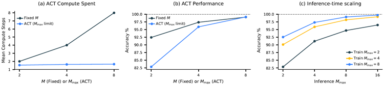
Figure 5 presents a performance comparison between two HRM variants: one incorporating ACT and another employing a fxed computational step count equivalent to ACT's \(M_{max}\) parameter. It shows that ACT effectively adapts its computational resources based on task complexity, achieving signifcant computational savings with minimal impact on performance.
図5は、ACTを組み込んだHRMバリアントと、ACTの \(M_{max}\) パラメータに相当する固定計算ステップ数を採用したHRMバリアントの2つのバリアントのパフォーマンス比較を示しています。ACTはタスクの複雑さに応じて計算リソースを効果的に調整し、パフォーマンスへの影響を最小限に抑えながら、大幅な計算コストの削減を実現していることがわかります。

Additional compute is especially effective for tasks that demand deeper reasoning. On Sudoku— a problem that often requires long-term planning—HRM exhibits strong inference-time scaling. On the other hand, we fnd that extra computational resources yield minimal gains in ARC-AGI challenge, as solutions generally require only a few transformations.
追加の計算リソースは、より深い推論を必要とするタスクに特に効果的です。長期的な計画が必要となることが多い数独問題では、HRMは推論時間に対して高いスケーリング効果を示します。一方、ARC-AGIチャレンジでは、解くのに通常わずかな変換しか必要としないため、追加の計算リソースによる効果は最小限であることがわかりました。

Figure 5: Effectiveness of Adaptive Computation Time (ACT) on the Sudoku-Extreme-Full. (a) Mean compute steps used by models with ACT versus models with a fxed number of compute steps (\(M\)). ACT maintains a low and stable number of average compute steps even as the maximum limit (\(M_{max}\)) increases. (b) Accuracy comparison. The ACT model achieves performance comparable to the fxed-compute model while utilizing substantially fewer computational steps on average. (c) Inference-time scalability. Models trained with a specifc \(M_{max}\) can generalize to higher computational limits during inference, leading to improved accuracy. For example, a model trained with \(M_{max} = 8\) continues to see accuracy gains when run with \(M_{max} = 16\) during inference.
図5: Sudoku-Extreme-Fullにおける適応型計算時間（ACT）の有効性。（a）ACT搭載モデルと固定計算ステップ数（\(M\)）のモデルで使用される平均計算ステップ数。ACTは、最大制限（\(M_{max}\)）が増加しても、平均計算ステップ数を低く安定させています。（b）精度の比較。ACTモデルは、平均して大幅に少ない計算ステップ数で、固定計算モデルに匹敵するパフォーマンスを実現しています。（c）推論時間のスケーラビリティ。特定の\(M_{max}\)でトレーニングされたモデルは、推論中により高い計算制限に一般化できるため、精度が向上します。たとえば、\(M_{max} = 8\)でトレーニングされたモデルは、推論中に\(M_{max} = 16\)で実行すると、精度が向上し続けます。

Stability of Q-learning in ACT　The deep Q-learning that underpins our ACT mechanism is known to be prone to instability, often requiring stabilization techniques such as replay buffers and target networks⁴⁸, which are absent in our design. Our approach, however, achieves stability through the intrinsic properties of our model and training procedure. Recent theoretical work by Gallici et al.⁴⁹ shows that Q-learning can achieve convergence if network parameters are bounded, weight decay is incorporated during training, and post-normalization layers are implemented. Our model satisfes these conditions through its Post-Norm architecture that employs RMSNorm (a layer normalization variant) and the AdamW optimizer. AdamW has been shown to solve an \(L_∞\)- constrained optimization problem, ensuring that model parameters remain bounded by \(1/λ\)⁵⁰.
ACT における Q 学習の安定性　ACT メカニズムの基盤となるディープ Q 学習は不安定になりやすいことが知られており、多くの場合、リプレイ バッファやターゲット ネットワーク⁴⁸ などの安定化手法が必要になりますが、私たちの設計ではこれらは使用されていません。しかし、私たちのアプローチでは、モデルとトレーニング手順の固有の特性によって安定性を実現しています。Gallici らによる最近の理論的研究⁴⁹ では、ネットワーク パラメータが制限され、トレーニング中に重み減衰が組み込まれ、ポスト正規化層が実装されている場合、Q 学習は収束を達成できることが示されています。私たちのモデルは、RMSNorm (層正規化のバリアント) と AdamW オプティマイザーを採用した Post-Norm アーキテクチャによってこれらの条件を満たしています。AdamW は、モデル パラメータが \(1/λ\) によって制限されたままになることを保証する、\(L_∞\) 制約の最適化問題を解決できることが示されています⁵⁰。

Architectural details　We employ a sequence-to-sequence architecture for HRM. Both input and output are represented as token sequences: \(x = (x_1,..., x_l)\) and \(y = (y_1,...,y_{l^\prime})\) respectively. The model includes an embedding layer \(f_I\) that converts discrete tokens into vector representa- tions, and an output head \(f_O(z;θ_O) = softmax(θ_Oz)\) that transforms hidden states into token prob- ability distributions \(\hat{y}\). For small-sample experiments, we replace softmax with stablemax51 to improve generalization performance. The sequence-to-sequence loss is averaged over all tokens,l \(LOSS(\hat{y}, y) = \frac{1}{l^\prime}\sum_{i=1}^{l^\prime} \log p(y_i)\), where \(p(y_i)\) is the probability that distribution \(\hat{y}_i\) assigns to token \(y_i\). The initial hidden states \(z^0\) are initialized by sampling from a truncated normal distribution with standard deviation of 1, truncation of 2, and kept fxed throughout training.
アーキテクチャの詳細　HRMにはsequence-to-sequenceアーキテクチャを採用しています。入力と出力はトークンシーケンスとして表現されます：\(x = (x_1,..., x_l)\)と\(y = (y_1,...,y_{l^\prime})\)。モデルには、離散トークンをベクトル表現に変換する埋め込み層\(f_I\)と、隠れ状態をトークン確率分布\(\hat{y}\)に変換する出力ヘッド\(f_O(z;θ_O) = softmax(θ_Oz)\)が含まれます。小規模サンプルの実験では、一般化性能を向上させるために、softmaxをstablemax51に置き換えます。シーケンス間損失はすべてのトークンについて平均化され、l \(LOSS(\hat{y}, y) = \frac{1}{l^\prime}\sum_{i=1}^{l^\prime} \log p(y_i)\) となります。ここで、\(p(y_i)\) は分布 \(\hat{y}_i\) がトークン \(y_i\) に割り当てる確率です。初期の隠れ状態 \(z^0\) は、標準偏差 1、切り捨て 2 の切断正規分布からサンプリングすることで初期化され、学習中は固定値に保たれます。

Both the low-level and high-level recurrent modules \(f_L\) and \(f_H\) are implemented using encoder- only Transformer⁵² blocks with identical architectures and dimensions. These modules take mul- tiple inputs, and we use straightforward element-wise addition to combine them, though more sophisticated merging techniques such as gating mechanisms could potentially improve perfor- mance and is left for future work. For all Transformer blocks in this work—including those in the baseline models—we incorporate the enhancements found in modern LLMs (based on Llama53 architectures). These improvements include Rotary Positional Encoding⁵⁴, Gated Linear Units⁵⁵, RMSNorm⁵⁶, and the removal of bias terms from linear layers.
低水準および高水準の再帰モジュール \(f_L\) と \(f_H\) はどちらも、同一のアーキテクチャおよび次元を持つエンコーダのみの Transformer⁵² ブロックを使用して実装されています。これらのモジュールは複数の入力を受け取り、それらを結合するために単純な要素ごとの加算を使用しますが、ゲーティングメカニズムなどのより洗練されたマージ手法は潜在的にパフォーマンスを向上させる可能性があり、将来の作業に残されています。本研究のすべての Transformer ブロック（ベースラインモデルのブロックを含む）には、最新の LLM（Llama53 アーキテクチャに基づく）に見られる機能強化が組み込まれています。これらの機能強化には、Rotary Positional Encoding⁵⁴、Gated Linear Units⁵⁵、RMSNorm⁵⁶、および線形層からのバイアス項の削除が含まれます。

Furthermore, both HRM and recurrent Transformer models implement a Post-Norm architecture with weights initialized via truncated LeCun Normal initialization^57,58,59, while the scale and bias parameters are excluded from RMSNorm. All parameters are optimized using the Adam-atan2 op- timizer⁶⁰, a scale-invariant variant of Adam⁶¹, combined with a constant learning rate that includes linear warm-up.
さらに、HRMモデルとリカレントTransformerモデルはどちらも、重みがTruncated LeCun Normal初期化法^57,58,59によって初期化されるPost-Normアーキテクチャを実装しています。一方、スケールパラメータとバイアスパラメータはRMSNormから除外されています。すべてのパラメータは、Adamのスケール不変版であるAdam-atan2最適化器⁶⁰と、線形ウォームアップを含む定数学習率を用いて最適化されます。⁶¹

3 Results 結果

This section begins by describing the ARC-AGI, Sudoku, and Maze benchmarks, followed by an overview of the baseline models and their results. Figure 6 -(a,b,c) presents a visual representa- tion of the three benchmark tasks, which are selected to evaluate various reasoning abilities in AI models.
このセクションでは、まずARC-AGI、数独、迷路のベンチマークについて説明し、続いてベースラインモデルとその結果の概要を説明します。図6 (a, b, c) は、AIモデルの様々な推論能力を評価するために選択された3つのベンチマークタスクを視覚的に表したものです。

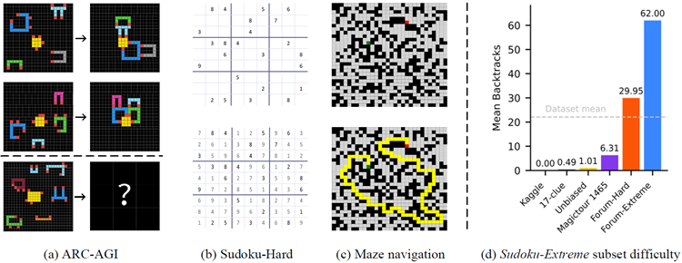
Figure 6: Left: Visualization of benchmark tasks. Right: Diffculty of Sudoku-Extreme examples.
図6: 左: ベンチマークタスクの視覚化。右: Sudoku-Extremeの例の難易度。

3.1 Benchmarks ベンチマーク

ARC-AGI Challenge　The ARC-AGI benchmark evaluates general fuid intelligence through IQ- test-like puzzles that require inductive reasoning²⁷. The initial version, ARC-AGI-1, presents chal- lenges as input-label grid pairs that force AI systems to extract and generalize abstract rules from just a few examples. Each task provides a few input–output demonstration pairs (usually 2–3) and a test input. An AI model has two attempts to produce the correct output grid. Although some be- lieve that mastering ARC-AGI would signal true artifcial general intelligence, its primary purpose is to expose the current roadblocks in AGI progress. In fact, both conventional deep learning meth- ods and CoT techniques have faced signifcant challenges with ARC-AGI-1, primarily because it requires the ability to generalize to entirely new tasks²⁸.
ARC-AGI チャレンジ　ARC-AGI ベンチマークは、帰納的推論を必要とする IQ テストのようなパズルを通じて、汎用流動知能を評価します²⁷。最初のバージョンである ARC-AGI-1 では、入力とラベルのグリッドのペアとして課題が提示され、AI システムはわずかな例から抽象的なルールを抽出して一般化する必要があります。各タスクでは、いくつかの入力と出力のデモンストレーション ペア (通常 2～3 個) とテスト入力が提供されます。AI モデルは、正しい出力グリッドを生成するために 2 回試行します。ARC-AGI を習得すれば真の汎用人工知能が実現すると考える人もいますが、その主な目的は、AGI の進歩における現在の障害を明らかにすることです。実際、従来のディープラーニング手法と CoT 技術の両方が、ARC-AGI-1 で大きな課題に直面しています。これは主に、まったく新しいタスクに一般化する能力が必要になるためです²⁸。

Addressing the limitations identifed in ARC-AGI-1, ARC-AGI-2 signifcantly expands the bench- mark by providing a more comprehensive and carefully refned collection of tasks. These new tasks emphasize deeper compositional reasoning, multi-step logic, contextual rule application, and symbolic abstraction. Human calibration studies show these tasks are challenging but doable for people, while being much harder for current AI systems, offering a clearer measure of general reasoning abilities²⁹.
ARC-AGI-2は、ARC-AGI-1で特定された限界に対処し、より包括的かつ綿密に改良されたタスク群を提供することで、ベンチマークを大幅に拡張します。これらの新しいタスクは、より深い構成的推論、多段階の論理、文脈的ルールの適用、そして記号的抽象化を重視しています。人間を対象としたキャリブレーション研究では、これらのタスクは人間にとっては困難ではあるものの実行可能である一方、現在のAIシステムにとってははるかに困難であることが示されており、一般的な推論能力をより明確に測定できます²⁹。

Sudoku-Extreme　Sudoku is a 9×9 logic puzzle, requiring each row, column, and 3×3 block to contain the digits 1–9 exactly once. A prediction is considered correct if it exactly matches the puzzle's unique solution. Sudoku's complex logical structure makes it a popular benchmark for evaluating logical reasoning in machine learning^62,63,64.
数独エクストリーム　数独は9×9の論理パズルで、各行、各列、3×3のブロックに1から9までの数字が1つずつ含まれている必要があります。予測がパズルの唯一の解と完全に一致した場合、正解とみなされます。数独の複雑な論理構造は、機械学習における論理的推論を評価するためのベンチマークとして広く使用されています^62,63,64。

The most frequently used Sudoku dataset in research, namely the Kaggle dataset65, can be fully solved using elementary single-digit techniques⁶⁶. The minimal 17-clue puzzles⁶², another widely- used collection, might seem more challenging due to its small number of clues. However, this perception is misleading—since 17 represents the minimum number of clues required to guarantee a unique Sudoku solution, these hints need to be highly orthogonal to each other. This orthogonal arrangement leads to many direct, easily-resolved solution paths⁶⁷.
研究で最も頻繁に利用されている数独データセット、すなわちKaggleデータセット65は、初歩的な1桁の数字を用いた技法を用いて完全に解くことができます⁶⁶。もう一つの広く利用されているデータセットである、最小17個のヒントパズル⁶²は、ヒントの数が少ないため、より難しそうに見えるかもしれません。しかし、この認識は誤解を招きます。17個は、数独の解が一意であることを保証するのに必要な最小のヒント数であるため、これらのヒントは互いに高度に直交している必要があります。この直交配置により、多くの直接的で簡単に解ける解の経路が生まれます⁶⁷。

We introduce Sudoku-Extreme, a more challenging dataset that is compiled from the aforemen- tioned easy datasets as well as puzzles recognized by the Sudoku community as exceptionally diffcult for human players:
ここでは、前述の簡単なデータセットと、数独コミュニティで人間のプレイヤーにとって非常に難しいと認識されているパズルからコンパイルされた、より挑戦的なデータセットである Sudoku-Extreme を紹介します。

The compiled data then undergo a strict 90/10 train-test split, ensuring that the test set puzzles cannot be derived through equivalent transformations of any training samples. Sudoku-Extreme is a down-sampled subset of this data containing 1000 training examples. We use Sudoku-Extreme in our main experiments (Figure 1 ), which focuses on small-sample learning scenarios. To guarantee convergence and control overftting effects in our analysis experiments (Figures 2 , 3 and 5 ), we use the complete training data, Sudoku-Extreme-Full, containing 3 831 994 examples.
コンパイルされたデータは、厳密に90/10のトレーニング/テスト分割を受け、テストセットのパズルがトレーニングサンプルの等価変換によって導出されないようにします。Sudoku-Extremeは、このデータのダウンサンプリングされたサブセットで、1000個のトレーニングサンプルが含まれています。私たちは、小規模サンプル学習シナリオに焦点を当てたメインの実験（図1）でSudoku-Extremeを使用しています。分析実験（図2、図3、図5）では、収束を保証し、過剰学習の影響を制御するために、3,831,994個のサンプルを含む完全なトレーニングデータであるSudoku-Extreme-Fullを使用しています。

We measure puzzle diffculty by counting the number of search backtracks (“guesses”) required by a smart Sudoku solver program tdoku, which uses propositional logic to reduce the number of guesses⁶⁷. Our Sudoku-Extreme dataset exhibits a mean diffculty of 22 backtracks per puzzle, sig- nifcantly higher than existing datasets, including recent handmade puzzles Sudoku-Bench⁶⁸ which average just 0.45 backtracks per puzzle. These subset complexity levels are shown in Figure 6 -(d).
パズルの難易度は、スマートな数独解答プログラムtdokuが要求する探索バックトラック（「推測」）の数を数えることで測定します。tdokuは命題論理を用いて推測回数を削減します⁶⁷。私たちのSudoku-Extremeデータセットは、パズルあたり平均22回のバックトラックという難易度を示しており、これは、パズルあたり平均0.45回のバックトラックしか必要としない最近の手作りパズルであるSudoku-Bench⁶⁸を含む既存のデータセットよりも大幅に高い数値です。これらのサブセットの複雑さのレベルは、図6-(d)に示されています。

Maze-Hard　This task involves fnding the optimal path in a 30×30 maze, making it interpretable and frequently used for training LLMs in search tasks^69,70,71. We adopt the instance generation procedure of Lehnert et al.⁷¹, but introduce an additional flter to retain only those instances whose diffculty exceeds 110. Here, “diffculty” is defned as the length of the shortest path, which aligns with the linear time complexity of the wavefront breadth-frst search algorithm on GPUs⁷². A path is considered correct if it is valid and optimal—that is, the shortest route from the start to the goal. The training and test set both include 1000 examples.
Maze-Hard このタスクでは、30×30 の迷路で最適な経路を見つけることが求められます。これにより、経路は解釈可能となり、探索タスクにおける LLM のトレーニングに頻繁に使用されます^69,70,71。私たちは Lehnert らのインスタンス生成手順を採用していますが⁷¹、難易度が 110 を超えるインスタンスのみを保持するための追加のフィルターを導入しています。ここで、「難易度」は最短経路の長さとして定義され、GPU 上の波面幅優先探索アルゴリズムの線形時間計算量と一致しています⁷²。経路が有効かつ最適である場合、つまりスタートからゴールまでの最短ルートである場合、その経路は正しいとみなされます。トレーニング セットとテスト セットの両方に 1000 個の例が含まれています。

3.2 Evaluation Details 評価の詳細

For all benchmarks, HRM models were initialized with random weights and trained in the sequence- to-sequence setup using the input-output pairs. The two-dimensional input and output grids were fattened and then padded to the maximum sequence length. The resulting performance is shown in Figure 1 . Remarkably, HRM attains these results with just ~1000 training examples per task—and without pretraining or CoT labels.
全てのベンチマークにおいて、HRMモデルはランダムな重みで初期化され、入力-出力ペアを用いてシーケンスツーシーケンス方式で学習されました。2次元の入力グリッドと出力グリッドは太らせられ、その後、最大シーケンス長までパディングされました。その結果得られたパフォーマンスを図1に示します。驚くべきことに、HRMはタスクごとにわずか約1000個の学習例で、事前学習やCoTラベルなしでこれらの結果を達成しました。

For ARC-AGI challenge, we start with (1) all demonstration and test input-label pairs from the training set, and (2) all demonstration pairs along with test inputs from the evaluation set. The dataset is augmented by applying translations, rotations, fips, and color permutations to the puz- zles. Each task example is prepended with a learnable special token that represents the puzzle it belongs to. At test time, we proceed as follows for each test input in the evaluation set: (1) Gener- ate and solve 1000 augmented variants and, for each, apply the inverse-augmentation transform to obtain a prediction. (2) Choose the two most popular predictions as the fnal outputs.³ All reported results are obtained by comparing the outputs with the withheld test labels from the evaluation set.
ARC-AGIチャレンジでは、（1）トレーニングセットのすべてのデモンストレーションとテストの入力ラベルのペア、および（2）評価セットのすべてのデモンストレーションのペアとテスト入力から開始します。データセットは、パズルに平行移動、回転、FIP、および色の順列を適用することで拡張されます。各タスクの例の先頭には、それが属するパズルを表す学習可能な特別なトークンが付加されます。テスト時には、評価セットの各テスト入力に対して次のように進めます。（1）1000個の拡張バリアントを生成して解き、それぞれに対して逆拡張変換を適用して予測を取得します。（2）最終出力として、最も人気のある2つの予測を選択します。³ 報告された結果はすべて、評価セットから差し控えられたテストラベルと出力を比較することによって得られます。

³ The ARC-AGI allows two attempts for each test input.
ARC-AGI では、テスト入力ごとに 2 回の試行が許可されます。

We augment Sudoku puzzles by applying band and digit permutations, while data augmentation is disabled for Maze tasks. Both tasks undergo only a single inference pass.
数独パズルにはバンドと数字の順列を適用することで拡張しますが、迷路タスクではデータ拡張は無効です。どちらのタスクも推論パスは1回のみ実行されます。

For ARC-AGI, the scores of the CoT models are taken from the offcial leaderboard²⁹, while for Sudoku and Maze, the scores are obtained by evaluating through the corresponding API.
ARC-AGI の場合、CoT モデルのスコアは公式リーダーボード²⁹ から取得されますが、数独と迷路の場合、スコアは対応する API を通じて評価することによって取得されます。

In Figure 1 , the baselines are grouped based on whether they are pre-trained and use CoT, or neither. The “Direct pred” baseline means using “direct prediction without CoT and pre-training”, which retains the exact training setup of HRM but swaps in a Transformer architecture. Interestingly, on ARC-AGI-1, “Direct pred” matches the performance of Liao and Gu⁷³, who built a carefully de- signed, domain-specifc equivariant network for learning the ARC-AGI task from scratch, without pre-training. By substituting the Transformer architecture with HRM's hierarchical framework and implementing ACT, we achieve more than a twofold performance improvement.
図1では、ベースラインは、事前学習済みでCoTを使用しているか、どちらも使用していないかに基づいてグループ分けされています。「Direct pred」ベースラインは、「CoTと事前学習なしの直接予測」を使用することを意味します。これは、HRMの学習設定を正確に維持しながら、Transformerアーキテクチャに置き換えます。興味深いことに、ARC-AGI-1では、「Direct pred」はLiaoとGu⁷³のパフォーマンスと一致します。彼らは、ARC-AGIタスクを事前学習なしでゼロから学習するために、慎重に設計されたドメイン固有の等変ネットワークを構築しました。TransformerアーキテクチャをHRMの階層型フレームワークに置き換え、ACTを実装することで、2倍以上のパフォーマンス向上を実現します。

On the Sudoku-Extreme and Maze-Hard benchmarks, the performance gap between HRM and the baseline methods is signifcant, as the baselines almost never manage to solve the tasks. These benchmarks that demand lengthy reasoning traces are particularly diffcult for CoT-based methods. With only 1000 training examples, the “Direct pred” baseline—which employs an 8-layer Trans- former identical in size to HRM—fails entirely on these challenging reasoning problems. When trained on the larger Sudoku-Extreme-Full dataset, however, “Direct pred” can solve some easy Sudoku puzzles and reaches 16.9% accuracy (see Figure 2 ). Lehnert et al.⁷¹ showed that a large vanilla Transformer model with 175M parameters, trained on 1 million examples across multiple trials, achieved only marginal success on 30x30 Maze tasks, with accuracy below 20% using the pass@64 evaluation metric.
Sudoku-ExtremeとMaze-Hardのベンチマークでは、HRMとベースライン手法のパフォーマンス差は顕著で、ベースライン手法ではこれらのタスクをほとんど解くことができません。長い推論トレースを必要とするこれらのベンチマークは、CoTベースの手法にとって特に困難です。わずか1000件のトレーニング例では、HRMと同等のサイズの8層Transformerを採用した「Direct pred」ベースラインは、これらの難しい推論問題に全く対応できません。しかし、より大規模なSudoku-Extreme-Fullデータセットでトレーニングすると、「Direct pred」は簡単な数独パズルを解くことができ、16.9%の精度に達します（図2参照）。 Lehnert ら⁷¹は、1 億 7,500 万のパラメータを持つ大規模な標準の Transformer モデルを複数の試行にわたって 100 万のサンプルでトレーニングした結果、30x30 Maze タスクでわずかに成功し、pass@64 評価メトリックを使用した精度は 20% 未満であったことを示しました。

3.3 Visualization of intermediate timesteps 中間タイムステップの可視化

Although HRM demonstrates strong performance on complex reasoning tasks, it raises an intrigu- ing question: what underlying reasoning algorithms does the HRM neural network actually imple- ment? Addressing this question is important for enhancing model interpretability and developing a deeper understanding of the HRM solution space.
HRMは複雑な推論タスクにおいて優れたパフォーマンスを発揮しますが、興味深い疑問が生じます。HRMニューラルネットワークは実際にはどのような推論アルゴリズムを実装しているのでしょうか？この疑問に取り組むことは、モデルの解釈可能性を高め、HRMソリューション空間への理解を深める上で重要です。

While a defnitive answer lies beyond our current scope, we begin our investigation by analyzing state trajectories and their corresponding solution evolution. More specifcally, at each timestep \(i\) and given the low-level and high-level state pair (\(z_L^i\) and \(z_H^i\)) we perform a preliminary forward pass through the \(H\)-module to obtain \(\overline{z}^i = f_H(z_H^i, z_L^i;θ_H)\) and its corresponding decoded prediction \(\overline{y}^i = f_O(\overline{z}^i;θ_O)\). The prediction \(\overline{y}^i\) is then visualized in Figure 7 .
決定的な答えは現時点では私たちの範囲外ですが、まずは状態軌跡とそれに対応する解の進化を分析することから調査を始めます。具体的には、各タイムステップ \(i\) において、低レベルと高レベルの状態ペア (\(z_L^i\) と \(z_H^i\)) が与えられた場合、\(H\) モジュールを予備的にフォワードパスして、\(\overline{z}^i = f_H(z_H^i, z_L^i;θ_H)\) と、それに対応するデコードされた予測値 \(\overline{y}^i = f_O(\overline{z}^i;θ_O)\) を取得します。予測値 \(\overline{y}^i\) は図 7 に視覚化されています。

Figure 7: Visualization of intermediate predictions by HRM on benchmark tasks. Top: Maze- Hard—blue cells indicate the predicted path. Middle: Sudoku-Extreme—bold cells represent ini- tial givens; red highlights cells violating Sudoku constraints; grey shading indicates changes from the previous timestep. Bottom: ARC-AGI-2 Task—left: provided example input-output pair; right: intermediate steps solving the test input.
図7: ベンチマークタスクにおける HRM による中間予測の視覚化。上: Maze-Hard - 青いセルは予測パスを示します。中央: Sudoku-Extreme - 太字のセルは初期条件、赤は Sudoku の制約に違反するセル、灰色の網掛けは前のタイムステップからの変更を示します。下: ARC-AGI-2 タスク - 左: 提供された入力と出力のペアの例、右: テスト入力を解く中間ステップ。

In the Maze task, HRM appears to initially explore several potential paths simultaneously, subse- quently eliminating blocked or ineffcient routes, then constructing a preliminary solution outline followed by multiple refnement iterations. In Sudoku, the strategy resembles a depth-frst search approach, where the model appears to explore potential solutions and backtracks when it hits dead ends. HRM uses a different approach for ARC tasks, making incremental adjustments to the board and iteratively improving it until reaching a solution. Unlike Sudoku, which involves frequent backtracking, the ARC solution path follows a more consistent progression similar to hill-climbing optimization.
迷路課題では、HRMは最初に複数の潜在的な経路を同時に探索し、その後、閉塞した経路や非効率的な経路を排除し、暫定的な解のアウトラインを構築した後、複数回の改良反復を行うようです。数独では、この戦略は深さ優先探索アプローチに似ており、モデルは潜在的な解を探索し、行き止まりにぶつかるとバックトラックするようです。ARC課題ではHRMは異なるアプローチを採用し、ボードに段階的な調整を加え、解に到達するまで反復的に改善していきます。頻繁なバックトラックを伴う数独とは異なり、ARCの解の経路は、山登り最適化に似た、より一貫した進行を辿ります。

Importantly, the model shows that it can adapt to different reasoning approaches, likely choosing an effective strategy for each particular task. Further research is needed to gain more comprehensive insights into these solution strategies.
重要なのは、このモデルが様々な推論アプローチに適応し、それぞれのタスクに効果的な戦略を選択できることを示していることです。これらの解決戦略に関するより包括的な洞察を得るには、さらなる研究が必要です。

4 Brain Correspondence 脳の対応

A key principle from systems neuroscience is that a brain region's functional repertoire—its ability to handle diverse and complex tasks—is closely linked to the dimensionality of its neural represen- tations^75,76. Higher-order cortical areas, responsible for complex reasoning and decision-making, must handle a wide variety of tasks, demanding more fexible and context-dependent processing⁷⁷. In dynamical systems, this fexibility is often realized through higher-dimensional state-space tra- jectories, which allow for a richer repertoire of potential computations⁷⁸. This principle gives rise to an observable dimensionality hierarchy, where a region's position in the processing hierarchy correlates with its effective dimensionality. To quantify this phenomenon, we can examine the Participation Ratio (PR), which serves as a standard measure of the effective dimensionality of a high-dimensional representation⁷⁹. The PR is calculated using the formula
システム神経科学の重要な原理は、脳領域の機能レパートリー（多様で複雑なタスクを処理する能力）は、その神経表現の次元数と密接に関連しているというものです^75,76。複雑な推論と意思決定を担う高次皮質領域は、多様なタスクを処理する必要があり、より柔軟で文脈依存的な処理が求められます⁷⁷。動的システムでは、この柔軟性は多くの場合、より豊富な潜在的計算レパートリーを可能にする高次元状態空間軌跡を通じて実現されます⁷⁸。この原理は、観測可能な次元階層を生み出し、処理階層における領域の位置はその実効次元数と相関します。この現象を定量化するために、高次元表現の実効次元数の標準的な尺度として機能する参加率（PR）を調べることができます⁷⁹。 PRは次の式で計算されます \[ PR =\frac{(\sum_i \lambda_i)^2}{\sum_i\lambda_i^2} \] where {\(λ_i\)} are the eigenvalues of the covariance matrix of neural trajectories. Intuitively, a higher PR value signifes that variance is distributed more evenly across many dimensions, corresponding to a higher-dimensional representation. Conversely, a lower PR value indicates that variance is concentrated in only a few principal components, refecting a more compact, lower-dimensional structure.
ここで、{\(λ_i\)}はニューラルトラジェクトリの共分散行列の固有値です。直感的に、PR値が高いほど、分散が多くの次元にわたってより均等に分布していることを意味し、高次元表現に対応します。逆に、PR値が低いほど、分散が少数の主成分に集中していることを意味し、よりコンパクトで低次元な構造を反映しています。

The dimensionality hierarchy can be observed, for example, in the mouse cortex, where the PR of population activity increases monotonically from low-level sensory areas to high-level associative areas, supporting this link between dimensionality and functional complexity⁷⁴ (Figure 8 (a,b)).
次元階層は、例えばマウスの皮質で観察することができ、集団活動のPRは、低レベルの感覚領域から高レベルの連合領域にかけて単調に増加しており、次元と機能的複雑さの間のこの関連を裏付けています⁷⁴（図8（a、b））。

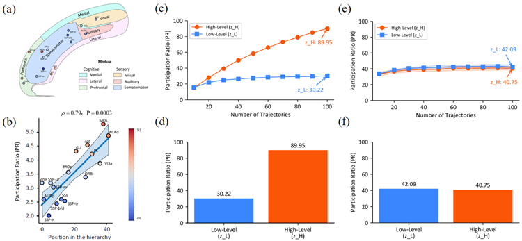
Figure 8: Hierarchical Dimensionality Organization in the HRM and Mouse Cortex. (a,b) are adapted from Posani et al.⁷⁴. (a) Anatomical illustration of mouse cortical areas, color-coded by functional modules. (b) Correlation between Participation Ratio (PR), a measure of effective neural dimensionality, and hierarchical position across different mouse cortical areas. Higher positions in the hierarchy (e.g., MOs, ACAd) exhibit signifcantly higher PR values compared to lower sensory areas (e.g., SSp-n), with a Spearman correlation coeffcient of ρ = 0.79 (P = 0.0003). (c,d) Trained HRM. (c) PR scaling of the trained HRM with task diversity. The dimensionality of the high- level module (\(z_H\)) scales with the number of unique tasks (trajectories) included in the analysis, indicating an adaptive expansion of its representational capacity. In contrast, the low-level module's (\(z_L\)) dimensionality remains stable. (d) PR values for the low-level (\(z_L\), PR = 30.22) and high- level (\(z_H\), PR = 89.95) modules of the trained HRM, computed from neural activity during 100 unique Sudoku-solving trajectories. A clear dimensionality hierarchy is observed, with the high- level module operating in a substantially higher-dimensional space. (e,f) Analysis of Untrained Network. To verify that the dimensionality hierarchy is an emergent property of training, the same analyses were performed on an untrained HRM with random weights. (e) In contrast to the trained model's scaling in (c), the dimensionality of both modules in the untrained model remains low and stable, failing to scale with the number of tasks. (f) Similarly, contrasting with the clear separation in (d), the PR values for the untrained model's modules (\(z_L\), PR = 42.09; \(z_H\), PR = 40.75) are low and nearly identical, showing no evidence of hierarchical separation. This confrms that the observed hierarchical organization of dimensionality is a learned property that emerges through training, not an artifact of the model's architecture.
図8：HRMとマウス皮質における階層的次元構造。（a、b）はPosaniら⁷⁴から引用。（a）機能モジュールごとに色分けしたマウス皮質領域の解剖図。（b）有効神経次元の尺度である参加率（PR）と、異なるマウス皮質領域間の階層的位置との相関。階層内の上位位置（MO、ACAdなど）は、下位の感覚領域（SSp-nなど）と比較して、有意に高いPR値を示し、スピアマン相関係数はρ = 0.79（P = 0.0003）であった。（c、d）訓練されたHRM。（c）タスクの多様性による訓練されたHRMのPRスケーリング。高レベルモジュール (\(z_H\)) の次元性は、分析に含まれる一意のタスク (軌跡) の数に応じて変化し、その表現能力が適応的に拡張されていることを示しています。対照的に、低レベルモジュール (\(z_L\)) の次元性は安定しています。(d) トレーニング済み HRM の低レベルモジュール (\(z_L\)、PR = 30.22) と高レベルモジュール (\(z_H\)、PR = 89.95) の PR 値。100 個の一意の数独を解く軌跡中の神経活動から計算されています。明確な次元階層が見られ、高レベルモジュールは大幅に高次元の空間で動作しています。(e、f) 未トレーニングネットワークの分析。次元階層がトレーニングの出現特性であることを確認するために、ランダムな重みを持つ未トレーニング HRM に対して同じ分析を実行しました。 (e) (c) の学習済みモデルのスケーリングとは対照的に、未学習モデルの両モジュールの次元数は低く安定しており、タスク数に応じてスケーリングできません。(f) 同様に、(d) の明確な分離とは対照的に、未学習モデルのモジュールの PR 値 (\(z_L\), PR = 42.09; \(z_H\), PR = 40.75) は低く、ほぼ同一であり、階層的な分離の証拠は見られません。これは、観察された次元の階層構造が、学習を通じて獲得された特性であり、モデルのアーキテクチャによる結果ではないことを裏付けています。

We evaluated whether HRM reproduces this neuroscientifc principle by calculating the PR for both recurrent modules after training on the Sudoku-Extreme Full dataset. The PR computation used the covariance matrix derived from neural states gathered across multiple Sudoku-solving trajectories. The results show a striking parallel to the biological fndings. The low-level module's state (\(z_L\)) occupies a relatively small subspace with a participation ratio of 30.22, whereas the high- level module's state (\(z_H\)) operates in a substantially larger subspace with a participation ratio of 89.95, as shown in Figure 8 (c). Furthermore, Figure 8 (d) shows that increasing the number of unique tasks (trajectories) from 10 to 100 causes \(z_H\) dimensionality to scale up accordingly, while \(z_L\) dimensionality remains stable. These results suggest an emergent separation of representational capacity between the modules that parallels their functional roles.
HRM がこの神経科学的原理を再現するかどうかを、Sudoku-Extreme Full データセットでトレーニングした後、両方のリカレント モジュールの PR を計算することで評価しました。PR の計算には、複数の数独を解く軌跡から収集された神経状態から得られた共分散行列を使用しました。結果は、生物学的な発見との顕著な類似点を示しています。図 8 (c) に示すように、低レベル モジュールの状態 (\(z_L\)) は、参加率が 30.22 の比較的小さなサブスペースを占めますが、高レベル モジュールの状態 (\(z_H\)) は、参加率が 89.95 のかなり大きなサブスペースで動作します。さらに、図 8 (d) は、一意のタスク (軌跡) の数を 10 から 100 に増やすと、\(z_H\) の次元がそれに応じてスケールアップしますが、\(z_L\) の次元は安定していることを示しています。これらの結果は、モジュール間の機能的役割と並行する表現能力の分離が出現したことを示唆しています。

To confrm that this hierarchical organization is an emergent property of training, and not an artifact of the network's architecture, we performed a control analysis using an identical but untrained network with random weights.
この階層構造がトレーニングによって生じた特性であり、ネットワークのアーキテクチャによる結果ではないことを確認するために、ランダムな重みを持つ同一だが未トレーニングのネットワークを使用して制御分析を実行しました。

We initialized an identical HRM architecture with random weights and, without any training, mea- sured the PR of its modules as the network processed the same task-specifc inputs given to the trained model.
我々はランダムな重みを持つ同一のHRMアーキテクチャを初期化し、訓練なしで、訓練されたモデルに与えられた同じタスク固有の入力をネットワークが処理するときのそのモジュールのPRを測定しました。

The results, shown in Figure 8 (e,f), reveal a stark contrast: the high-level and low-level modules of the untrained network exhibit no hierarchical separation, with their PR values remaining low and nearly indistinguishable from each other. This control analysis validates that the dimensionality hierarchy is an emergent property that arises as the model learns to perform complex reasoning.
図8（e, f）に示す結果は、際立った対照を示しています。未学習ネットワークの高レベルモジュールと低レベルモジュールは階層的な分離を示さず、PR値は低いままで、互いにほとんど区別がつきません。この制御分析は、次元階層が、モデルが複雑な推論を実行することを学習するにつれて生じる創発的な特性であることを検証しています。

The high-to-low PR ratio in HRM (\(z_H/z_L \approx 2.98\)) closely matches that measured in the mouse cortex (\(\approx 2.25\)). In contrast, conventional deep networks often exhibit neural collapse, where last-layer features converge to a low-dimensional subspace^80,81,82. HRM therefore departs from the collapse pattern and instead fosters a high-dimensional representation in its higher module. This is signifcant because such representations are considered crucial for cognitive fexibility and are a hallmark of higher-order brain regions like the prefrontal cortex (PFC), which is central to complex reasoning.
HRMにおける高低PR比（\(z_H/z_L \approx 2.98\)）は、マウス大脳皮質で測定された値（\(\approx 2.25\)）とほぼ一致しています。対照的に、従来の深層ネットワークでは、最終層の特徴が低次元部分空間に収束する神経崩壊がしばしば見られます^80,81,82。したがって、HRMはこのような崩壊パターンから逸脱し、代わりに高次モジュールにおいて高次元表現を促進します。これは、このような表現が認知の柔軟性に不可欠であると考えられており、複雑な推論の中核を担う前頭前野（PFC）などの高次脳領域の特徴であるため、重要です。

This structural parallel suggests the model has discovered a fundamental organizational principle. By learning to partition its representations into a high-capacity, high-dimensional subspace (\(z_H\)) and a more specialized, low-dimensional one (\(z_L\)), HRM autonomously discovers an organizational principle that is thought to be fundamental for achieving robust and fexible reasoning in biological systems. This provides a potential mechanistic explanation for the model's success on complex, long-horizon tasks that are intractable for models lacking such a differentiated internal structure. We emphasize, however, that this evidence is correlational. While a causal link could be tested via intervention (e.g., by constraining the \(H\)-module's dimensionality), such methods are diffcult to interpret in deep learning due to potential confounding effects on the training process itself. Thus, the causal necessity of this emergent hierarchy remains an important question for future investigation.
この構造的な類似性は、モデルが根本的な組織化原理を発見したことを示唆しています。HRMは、その表現を大容量・高次元の部分空間 (\(z_H\)) と、より特化した低次元の部分空間 (\(z_L\)) に分割することを学習することで、生物系において堅牢かつ柔軟な推論を実現するために不可欠と考えられる組織化原理を自律的に発見します。これは、このような差別化された内部構造を持たないモデルでは扱いにくい、複雑で長期的なタスクにおいて、モデルが成功していることのメカニズム的な説明となる可能性があります。ただし、この証拠は相関関係に基づくものであることを強調しておきます。因果関係は介入（例えば、\(H\)モジュールの次元数を制限すること）によって検証できますが、深層学習においては、トレーニングプロセス自体に潜在的な交絡効果が生じる可能性があるため、そのような手法を解釈することは困難です。したがって、この新たな階層構造の因果的必然性は、今後の研究における重要な問題として残されています。

5 Related Work 関連研究

Reasoning and algorithm learning　Given the central role of reasoning problems and their close relation to algorithms, researchers have long explored neural architectures that enable algorithm learning from training instances. This line of work includes Neural Turing Machines (NTM)⁸³, the Differentiable Neural Computer (DNC)⁸⁴, and Neural GPUs⁸⁵–all of which construct iterative neural architectures that mimic computational hardware for algorithm execution, and are trained to learn algorithms from data. Another notable work in this area is Recurrent Relational Networks (RRN)⁶², which executes algorithms on graph representations through graph neural networks.
推論とアルゴリズム学習　推論問題が中心的な役割を果たし、アルゴリズムと密接に関連していることから、研究者は長年、トレーニングインスタンスからアルゴリズムを学習できるニューラルアーキテクチャを研究してきました。この研究分野には、ニューラルチューリングマシン（NTM）⁸³、微分可能ニューラルコンピュータ（DNC）⁸⁴、ニューラルGPU⁸⁵が含まれます。これらはすべて、アルゴリズム実行用の計算ハードウェアを模倣した反復的なニューラルアーキテクチャを構築し、データからアルゴリズムを学習するようにトレーニングされます。この分野で注目すべきもう1つの研究は、グラフニューラルネットワークを介してグラフ表現上でアルゴリズムを実行するリカレントリレーショナルネットワーク（RRN）⁶²です。

Recent studies have integrated algorithm learning approaches with Transformer-based architec- tures. Universal Transformers extend the standard Transformer model by introducing a recurrent loop over the layers and implementing an adaptive halting mechanism. Geiping et al.⁸⁶ demonstrate that looped Transformers can generalize to a larger number of recurrent steps during inference than what they were trained on. Shen et al.¹⁶ propose adding continuous recurrent reasoning tokens to the Transformer. Finally, TransNAR⁸ combine recurrent graph neural networks with language models.
最近の研究では、アルゴリズム学習アプローチとTransformerベースのアーキテクチャが統合されています。Universal Transformerは、層に再帰ループを導入し、適応的な停止メカニズムを実装することで、標準的なTransformerモデルを拡張します。Geipingら⁸⁶は、ループされたTransformerが、推論中に訓練時よりも多くの再帰ステップに一般化できることを実証しました。Shenら¹⁶は、Transformerに連続的な再帰推論トークンを追加することを提案しています。最後に、TransNAR⁸は、再帰グラフニューラルネットワークと言語モデルを組み合わせています。

Building on the success of CoT-based reasoning, a line of work have introduced fne-tuning meth- ods that use reasoning paths from search algorithms (like A*) as SFT targets^87,71,70.
CoT ベースの推論の成功を基に、一連の研究では、検索アルゴリズム (A* など) からの推論パスを SFT ターゲットとして使用する微調整手法が導入されました^87,71,70。

We also mention adaptive halting mechanisms designed to allocate additional computational re- sources to more challenging problems. This includes the Adaptive Computation Time (ACT) for RNNs⁸⁸ and follow-up research like PonderNet⁸⁹, which aims to improve the stability of this allo- cation process.
また、より困難な問題に追加の計算リソースを割り当てるために設計された適応停止機構についても言及する。これには、RNNの適応計算時間（ACT）⁸⁸や、この割り当てプロセスの安定性を向上させることを目的としたPonderNet⁸⁹などの後継研究が含まれる。

HRM further pushes the boundary of algorithm learning through a brain-inspired computational architecture that achieves exceptional data effciency and model expressiveness, successfully dis- covering complex and diverse algorithms from just 1000 training examples.
HRM は、優れたデータ効率とモデル表現力を実現する脳にヒントを得た計算アーキテクチャを通じてアルゴリズム学習の限界をさらに押し広げ、わずか 1,000 のトレーニング例から複雑で多様なアルゴリズムを発見することに成功しました。

Brain-inspired reasoning architectures　Developing a model with the reasoning power of the brain has long been a goal in brain-inspired computing. Spaun⁹⁰ is one notable example, which uses spiking neural networks to create distinct modules corresponding to brain regions like the visual cortex and prefrontal cortex. This design enables an architecture to perform a range of cognitive tasks, from memory recall to simple reasoning puzzles. However, its reasoning relies on hand- designed algorithms, which may limit its ability to learn new tasks. Another signifcant model is the Tolman-Eichenbaum Machine (TEM)⁹¹, which is inspired by the hippocampal-entorhinal system's role in spatial and relational memory tasks. TEM proposes that medial entorhinal cells create a basis for structural knowledge, while hippocampal cells link this basis to sensory information. This allows TEM to generalize and explains the emergence of various cell types like grid, border, and place cells. Another approach involves neural sampling models⁹², which view the neural signaling process as inference over a distribution, functioning similarly to a Boltzmann machine. These models often require hand-made rules to be set up for solving a specifc reasoning task. In essence, while prior models are restricted to simple reasoning problems, HRM is designed to solve complex tasks that are hard for even advanced LLMs, without pre-training or task-specifc manual design.
脳に着想を得た推論アーキテクチャ　脳の推論能力を備えたモデルの開発は、脳に着想を得たコンピューティングの長年の目標でした。Spaun⁹⁰ は注目すべき例の 1 つで、スパイキング ニューラル ネットワークを使用して、視覚野や前頭前皮質などの脳領域に対応する個別のモジュールを作成します。この設計により、アーキテクチャは記憶の想起から単純な推論パズルまで、さまざまな認知タスクを実行できます。ただし、その推論は手動で設計されたアルゴリズムに依存しているため、新しいタスクを学習する能力が制限される可能性があります。もう 1 つの重要なモデルは、Tolman-Eichenbaum Machine (TEM)⁹¹ で、空間記憶と関係記憶タスクにおける海馬-嗅内皮質系の役割にヒントを得たものです。TEM では、内側嗅内皮質細胞が構造的知識の基礎を作成し、海馬細胞がこの基礎を感覚情報に結び付けると提唱されています。これにより、TEMはグリッド細胞、境界細胞、場所細胞といった様々な細胞タイプの出現を一般化し、説明することが可能になります。もう一つのアプローチとして、ニューラルサンプリングモデル⁹²が挙げられます。これは、神経シグナル伝達プロセスを分布に基づく推論と捉え、ボルツマンマシンと同様に機能します。これらのモデルでは、特定の推論タスクを解決するために、多くの場合、手作業でルールを設定する必要があります。本質的には、従来のモデルが単純な推論問題に限定されているのに対し、HRMは、事前学習やタスク固有の手動設計なしに、高度なLLMでさえ困難な複雑なタスクを解くように設計されています。

Hierarchical memory　The hierarchical multi-timescale structure also plays an important role in how the brain processes memory. Models such as Hierarchical Sequential Models⁹³ and Clockwork RNN⁹⁴ use multiple recurrent modules that operate at varying time scales to more effectively cap- ture long-range dependencies within sequences, thereby mitigating the forgetting issue in RNNs.
階層的記憶　階層的なマルチタイムスケール構造は、脳の記憶処理においても重要な役割を果たします。階層的シーケンシャルモデル⁹³やクロックワークRNN⁹⁴などのモデルは、様々な時間スケールで動作する複数の再帰モジュールを用いることで、シーケンス内の長期的な依存関係をより効果的に捉え、RNNにおける忘却の問題を軽減します。

Similar mechanisms have also been adopted in linear attention methods for memorizing long con- texts (see the Discussions section). Since HRM focuses on reasoning, full attention is applied for simplicity. Incorporating hierarchical memory into HRM could be a promising future direction.
同様のメカニズムは、長い文脈を記憶するための線形注意法にも採用されています（「考察」セクションを参照）。HRMは推論に重点を置いているため、簡略化のために完全な注意が適用されます。階層的記憶をHRMに組み込むことは、将来的に有望な方向性となる可能性があります。

6 Discussions 考察

Turing-completeness of HRM Like earlier neural reasoning algorithms including the Universal Transformer⁹⁵, HRM is computationally universal when given suffcient memory and time con- straints. In other words, it falls into the category of models that can simulate any Turing machine, overcoming the computational limitations of standard Transformers discussed previously in the in- troduction. Given that earlier neural algorithm reasoners were trained as recurrent neural networks, they suffer from premature convergence and memory intensive BPTT. Therefore, in practice, their effective computational depth remains limited, though still deeper than that of a standard Trans- former. By resolving these two challenges and being equipped with adaptive computation, HRM could be trained on long reasoning processes, solve complex puzzles requiring intensive depth-frst search and backtracking, and move closer to practical Turing-completeness.
HRM のチューリング完全性 Universal Transformer⁹⁵ などの以前のニューラル推論アルゴリズムと同様に、HRM は十分なメモリと時間の制約が与えられれば計算的にユニバーサルです。言い換えると、HRM は、導入で前述した標準的な Transformer の計算上の制限を克服し、あらゆるチューリング マシンをシミュレートできるモデルのカテゴリに分類されます。以前のニューラル アルゴリズム推論エンジンは再帰型ニューラル ネットワークとしてトレーニングされていたため、早期収束とメモリを大量に消費する BPTT に悩まされていました。そのため、実際には、有効な計算の深さは限られたままですが、それでも標準的な Transformer よりは深いです。これら 2 つの課題を解決し、適応型計算を備えることで、HRM は長い推論プロセスでトレーニングでき、集中的な深さ優先探索とバックトラッキングを必要とする複雑なパズルを解き、実用的なチューリング完全性に近づくことができます。

Reinforcement learning with chain-of-thought　Beyond fne-tuning using human-annotated CoT, reinforcement learning (RL) represents another widely adopted training methodology. However, recent evidence suggests that RL primarily unlocks existing CoT-like capabilities rather than dis- covering fundamentally new reasoning mechanisms^96,97,98,99. Additionally, CoT-training with RL is known for its instability and data ineffciency, often requiring extensive exploration and careful reward design. In contrast, HRM takes feedback from dense gradient-based supervision rather than relying on a sparse reward signal. Moreover, HRM operates naturally in a continuous space, which is biologically plausible and avoids allocating same computational resources to each token, even though tokens vary in their reasoning and planning complexity¹⁶.
思考の連鎖による強化学習　人間が注釈を付けたCoTを使用した微調整を超えて、強化学習（RL）はもう1つの広く採用されているトレーニング方法論です。しかし、最近の証拠は、RLが根本的に新しい推論メカニズムを発見するのではなく、主に既存のCoTのような機能を解放することを示唆しています^96,97,98,99。さらに、RLによるCoTトレーニングは不安定性とデータの非効率性で知られており、多くの場合、広範な探索と慎重な報酬設計が必要です。対照的に、HRMはスパースな報酬信号に頼るのではなく、稠密な勾配ベースの監督からフィードバックを受け取ります。さらに、HRMは連続空間で自然に動作します。これは生物学的に妥当であり、トークンの推論と計画の複雑さが異なっていても、各トークンに同じ計算リソースを割り当てることを回避します¹⁶。

Linear attention　Recurrence has been explored not only for its capability in universal computa- tion, but also as a means to replace the attention mechanism in Transformers, which suffers from quadratic time and memory complexity¹⁰⁰. Recurrent alternatives offer a more effcient design by processing input tokens sequentially and predicting the next token at each time step, similar to early RNN-based language models.
線形アテンション 再帰は、汎用的な計算能力だけでなく、Transformerのアテンション機構を置き換える手段としても研究されてきました。Transformerのアテンション機構は、計算時間とメモリの複雑度が2乗に比例します¹⁰⁰。再帰的な代替手法は、初期のRNNベースの言語モデルと同様に、入力トークンを順次処理し、各タイムステップで次のトークンを予測することで、より効率的な設計を提供します。

Some linear-attention variants, such as Log-linear Attention¹⁰¹, share an RNN-like state-update that can be interpreted as propagating multi-timescale summary statistics, thereby retaining long-range context without the quadratic memory growth of standard self-attention. However, substituting the attention mechanism alone does not change the fact that Transformers are still fxed-depth, and require CoT as a compensatory mechanism. Notably, linear attention can operate with a reduced key-value cache over extended contexts, making them more suitable for deployment on resource- constrained edge devices.
Log-linear Attention¹⁰¹ などの一部の線形アテンションの変種は、RNNのような状態更新を共有しており、これはマルチタイムスケールの要約統計を伝播するものと解釈できるため、標準的な自己アテンションのような二次的なメモリ増加なしに、長距離コンテキストを保持できます。しかし、アテンションメカニズムのみを置き換えても、Transformerが依然として固定深度であり、補償メカニズムとしてCoTを必要とするという事実は変わりません。特に、線形アテンションは拡張コンテキスト上でキーバリューキャッシュを削減して動作できるため、リソースが限られたエッジデバイスへの導入に適しています。

7 Conclusion 結論

This work introduces the Hierarchical Reasoning Model, a brain-inspired architecture that lever- ages hierarchical structure and multi-timescale processing to achieve substantial computational depth without sacrifcing training stability or effciency. With only 27M parameters and train- ing on just 1000 examples, HRM effectively solves challenging reasoning problems such as ARC, Sudoku, and complex maze navigation–tasks that typically pose signifcant diffculties for contem- porary LLM and chain-of-thought models.
本研究では、階層的推論モデル（Hierarchical Reasoning Model）を紹介します。これは、脳に着想を得たアーキテクチャで、階層構造とマルチタイムスケール処理を活用することで、学習の安定性や効率性を犠牲にすることなく、高い計算深度を実現します。わずか2,700万個のパラメータとわずか1,000個の例題を用いた学習で、Hierarchical Reasoning ModelはARC、数独、複雑な迷路ナビゲーションといった、現代のLLM（論理的思考モデル）や連鎖思考モデルでは通常大きな困難を伴う難問を効果的に解くことができます。

Although the brain relies heavily on hierarchical structures to enable most cognitive processes, these concepts have largely remained confned to academic literature rather than being translated into practical applications. The prevailing AI approach continues to favor non-hierarchical models. Our results challenge this established paradigm and suggest that the Hierarchical Reasoning Model represents a viable alternative to the currently dominant chain-of-thought reasoning methods, ad- vancing toward a foundational framework capable of Turing-complete universal computation.
脳はほとんどの認知プロセスを可能にするために階層構造に大きく依存していますが、これらの概念は主に学術文献の域に留まっており、実用化には至っていません。現在のAIアプローチは、依然として非階層的モデルを好んでいます。私たちの研究結果は、この確立されたパラダイムに異議を唱え、階層的推論モデルが現在主流となっている思考連鎖型推論手法に代わる現実的な選択肢となり、チューリング完全な普遍的計算を可能にする基礎的枠組みへと前進することを示唆しています。

Acknowledgements We thank Mingli Yuan, Ahmed Murtadha Hasan Mahyoub and Hengshuai Yao for their insightful discussions and valuable feedback throughout the course of this work.
謝辞 本研究の過程を通して洞察に満ちた議論と貴重なフィードバックを提供してくれた Mingli Yuan、Ahmed Murtadha Hasan Mahyoub、Hengshuai Yao に感謝します。

References 参考文献